Using Greenland Ice Mapping Project Data Tools + ICESat-2 Data
Contents
Using Greenland Ice Mapping Project Data Tools + ICESat-2 Data#
This notebook illustrates some of the various tools and capabilities available to access and explore imagery and velocity data products from the Greenland Ice Mapping Project GrIMP. Specifically, we will use the functionality of nisarVel and nisarVelSeries classes for working with GrIMP velocity products.
This notebook will also include examples of how to quickly explore imagery and velocity mosaics, formatted as cloud optimized GeoTIFF (more on that below) to interactively select and download subsets of GrIMP imagery (NSIDC-0723) and velocity (NSIDC-481, 0725, 0727, 0731, 0766) data. For the Sentinel-based velocity mosaics (0725, 0727, 0731), a user can select a box on a map and choose which components are downloaded (vv, vx, vy, ex, ey, dT) and saved to a netCDF file.
We will explore some of this functionality, read in and plot velocities over an area of interest, quickly run some statistical calculations to visualize how ice flow has changed, and also evaluate these changes in conjunction with the ICESat-2 ALL06 land ice elevation product.
Environment setup#
Generally, GrIMP notebooks use a set of tools that have been tested with the environment.yml in the binder folder of the GrIMP repository. Thus, for best results when using GrIMP notebooks in the future and in local instances, create a new conda environment to run this and other other GrIMP notebooks from this repository. After downloading the environment.yml file, enter the following commands at the command line to prepare your environment. For today’s tutorial in CryoCloud, we do not need to perform these steps.
conda env create -f binder/environment.yml
conda activate greenlandMapping
python -m ipykernel install --user --name=greenlandMapping
jupyter lab
See NSIDCLoginNotebook for additional information.
The notebooks can be run on a temporary virtual instance (to start click binder). See the github README for further details.
Note
In order to use the full functionality of GrIMP notebooks for this tutorial, we will pip install two two packages with functions for reading, subsetting, plotting, and downloading various datasets.
%pip install git+https://github.com/fastice/grimpfunc.git@master
%pip install git+https://github.com/fastice/nisardev.git@main
Collecting git+https://github.com/fastice/grimpfunc.git@master
  Cloning https://github.com/fastice/grimpfunc.git (to revision master) to /tmp/pip-req-build-uj62986d
  Running command git clone --filter=blob:none --quiet https://github.com/fastice/grimpfunc.git /tmp/pip-req-build-uj62986d
  Resolved https://github.com/fastice/grimpfunc.git to commit e65a24df129c9702be75209dd981a9748c8def49
  Installing build dependencies ... ?25ldone
?25h  Getting requirements to build wheel ... ?25ldone
?25h  Preparing metadata (pyproject.toml) ... ?25ldone
?25hRequirement already satisfied: holoviews<2,>=1 in /srv/conda/envs/notebook/lib/python3.10/site-packages (from grimpfunc==0.0.4) (1.17.0)
Requirement already satisfied: panel<1,>=0 in /srv/conda/envs/notebook/lib/python3.10/site-packages (from grimpfunc==0.0.4) (0.14.4)
Requirement already satisfied: stackstac<1,>=0 in /srv/conda/envs/notebook/lib/python3.10/site-packages (from grimpfunc==0.0.4) (0.4.4)
Requirement already satisfied: rio-stac<1,>=0 in /srv/conda/envs/notebook/lib/python3.10/site-packages (from grimpfunc==0.0.4) (0.8.0)
Requirement already satisfied: progressbar2<4,>=3 in /srv/conda/envs/notebook/lib/python3.10/site-packages (from grimpfunc==0.0.4) (3.55.0)
Requirement already satisfied: dask>=2021 in /srv/conda/envs/notebook/lib/python3.10/site-packages (from grimpfunc==0.0.4) (2022.11.0)
Requirement already satisfied: rioxarray<1,>=0 in /srv/conda/envs/notebook/lib/python3.10/site-packages (from grimpfunc==0.0.4) (0.14.1)
Requirement already satisfied: pandas<2,>=1 in /srv/conda/envs/notebook/lib/python3.10/site-packages (from grimpfunc==0.0.4) (1.5.1)
Requirement already satisfied: xarray>=0.20 in /srv/conda/envs/notebook/lib/python3.10/site-packages (from grimpfunc==0.0.4) (2023.7.0)
Requirement already satisfied: numpy<2,>=1 in /srv/conda/envs/notebook/lib/python3.10/site-packages (from grimpfunc==0.0.4) (1.23.5)
Requirement already satisfied: pystac<2,>=1 in /srv/conda/envs/notebook/lib/python3.10/site-packages (from grimpfunc==0.0.4) (1.8.2)
Requirement already satisfied: hvplot<1,>=0 in /srv/conda/envs/notebook/lib/python3.10/site-packages (from grimpfunc==0.0.4) (0.8.2)
Requirement already satisfied: requests<3,>=2 in /srv/conda/envs/notebook/lib/python3.10/site-packages (from grimpfunc==0.0.4) (2.31.0)
Requirement already satisfied: toolz>=0.8.2 in /srv/conda/envs/notebook/lib/python3.10/site-packages (from dask>=2021->grimpfunc==0.0.4) (0.12.0)
Requirement already satisfied: fsspec>=0.6.0 in /srv/conda/envs/notebook/lib/python3.10/site-packages (from dask>=2021->grimpfunc==0.0.4) (2022.11.0)
Requirement already satisfied: partd>=0.3.10 in /srv/conda/envs/notebook/lib/python3.10/site-packages (from dask>=2021->grimpfunc==0.0.4) (1.4.0)
Requirement already satisfied: cloudpickle>=1.1.1 in /srv/conda/envs/notebook/lib/python3.10/site-packages (from dask>=2021->grimpfunc==0.0.4) (2.2.1)
Requirement already satisfied: pyyaml>=5.3.1 in /srv/conda/envs/notebook/lib/python3.10/site-packages (from dask>=2021->grimpfunc==0.0.4) (6.0)
Requirement already satisfied: click>=7.0 in /srv/conda/envs/notebook/lib/python3.10/site-packages (from dask>=2021->grimpfunc==0.0.4) (8.1.6)
Requirement already satisfied: packaging>=20.0 in /srv/conda/envs/notebook/lib/python3.10/site-packages (from dask>=2021->grimpfunc==0.0.4) (23.1)
Requirement already satisfied: param<3.0,>=1.12.0 in /srv/conda/envs/notebook/lib/python3.10/site-packages (from holoviews<2,>=1->grimpfunc==0.0.4) (1.13.0)
Requirement already satisfied: pyviz-comms>=0.7.4 in /srv/conda/envs/notebook/lib/python3.10/site-packages (from holoviews<2,>=1->grimpfunc==0.0.4) (2.3.2)
Requirement already satisfied: colorcet in /srv/conda/envs/notebook/lib/python3.10/site-packages (from holoviews<2,>=1->grimpfunc==0.0.4) (3.0.1)
Requirement already satisfied: bokeh>=1.0.0 in /srv/conda/envs/notebook/lib/python3.10/site-packages (from hvplot<1,>=0->grimpfunc==0.0.4) (2.4.3)
Requirement already satisfied: python-dateutil>=2.8.1 in /srv/conda/envs/notebook/lib/python3.10/site-packages (from pandas<2,>=1->grimpfunc==0.0.4) (2.8.2)
Requirement already satisfied: pytz>=2020.1 in /srv/conda/envs/notebook/lib/python3.10/site-packages (from pandas<2,>=1->grimpfunc==0.0.4) (2023.3)
Requirement already satisfied: setuptools>=42 in /srv/conda/envs/notebook/lib/python3.10/site-packages (from panel<1,>=0->grimpfunc==0.0.4) (67.7.2)
Requirement already satisfied: pyct>=0.4.4 in /srv/conda/envs/notebook/lib/python3.10/site-packages (from panel<1,>=0->grimpfunc==0.0.4) (0.4.6)
Requirement already satisfied: typing-extensions in /srv/conda/envs/notebook/lib/python3.10/site-packages (from panel<1,>=0->grimpfunc==0.0.4) (4.6.3)
Requirement already satisfied: bleach in /srv/conda/envs/notebook/lib/python3.10/site-packages (from panel<1,>=0->grimpfunc==0.0.4) (6.0.0)
Requirement already satisfied: markdown in /srv/conda/envs/notebook/lib/python3.10/site-packages (from panel<1,>=0->grimpfunc==0.0.4) (3.4.4)
Requirement already satisfied: tqdm>=4.48.0 in /srv/conda/envs/notebook/lib/python3.10/site-packages (from panel<1,>=0->grimpfunc==0.0.4) (4.64.1)
Requirement already satisfied: python-utils>=2.3.0 in /srv/conda/envs/notebook/lib/python3.10/site-packages (from progressbar2<4,>=3->grimpfunc==0.0.4) (3.7.0)
Requirement already satisfied: six in /srv/conda/envs/notebook/lib/python3.10/site-packages (from progressbar2<4,>=3->grimpfunc==0.0.4) (1.16.0)
Requirement already satisfied: certifi>=2017.4.17 in /srv/conda/envs/notebook/lib/python3.10/site-packages (from requests<3,>=2->grimpfunc==0.0.4) (2023.5.7)
Requirement already satisfied: urllib3<3,>=1.21.1 in /srv/conda/envs/notebook/lib/python3.10/site-packages (from requests<3,>=2->grimpfunc==0.0.4) (1.26.15)
Requirement already satisfied: charset-normalizer<4,>=2 in /srv/conda/envs/notebook/lib/python3.10/site-packages (from requests<3,>=2->grimpfunc==0.0.4) (3.1.0)
Requirement already satisfied: idna<4,>=2.5 in /srv/conda/envs/notebook/lib/python3.10/site-packages (from requests<3,>=2->grimpfunc==0.0.4) (3.4)
Requirement already satisfied: rasterio in /srv/conda/envs/notebook/lib/python3.10/site-packages (from rio-stac<1,>=0->grimpfunc==0.0.4) (1.3.8)
Requirement already satisfied: pyproj>=2.2 in /srv/conda/envs/notebook/lib/python3.10/site-packages (from rioxarray<1,>=0->grimpfunc==0.0.4) (3.6.0)
Requirement already satisfied: pillow>=7.1.0 in /srv/conda/envs/notebook/lib/python3.10/site-packages (from bokeh>=1.0.0->hvplot<1,>=0->grimpfunc==0.0.4) (9.5.0)
Requirement already satisfied: tornado>=5.1 in /srv/conda/envs/notebook/lib/python3.10/site-packages (from bokeh>=1.0.0->hvplot<1,>=0->grimpfunc==0.0.4) (6.1)
Requirement already satisfied: Jinja2>=2.9 in /srv/conda/envs/notebook/lib/python3.10/site-packages (from bokeh>=1.0.0->hvplot<1,>=0->grimpfunc==0.0.4) (3.1.2)
Requirement already satisfied: locket in /srv/conda/envs/notebook/lib/python3.10/site-packages (from partd>=0.3.10->dask>=2021->grimpfunc==0.0.4) (1.0.0)
Requirement already satisfied: click-plugins in /srv/conda/envs/notebook/lib/python3.10/site-packages (from rasterio->rio-stac<1,>=0->grimpfunc==0.0.4) (1.1.1)
Requirement already satisfied: snuggs>=1.4.1 in /srv/conda/envs/notebook/lib/python3.10/site-packages (from rasterio->rio-stac<1,>=0->grimpfunc==0.0.4) (1.4.7)
Requirement already satisfied: affine in /srv/conda/envs/notebook/lib/python3.10/site-packages (from rasterio->rio-stac<1,>=0->grimpfunc==0.0.4) (2.4.0)
Requirement already satisfied: cligj>=0.5 in /srv/conda/envs/notebook/lib/python3.10/site-packages (from rasterio->rio-stac<1,>=0->grimpfunc==0.0.4) (0.7.2)
Requirement already satisfied: attrs in /srv/conda/envs/notebook/lib/python3.10/site-packages (from rasterio->rio-stac<1,>=0->grimpfunc==0.0.4) (21.4.0)
Requirement already satisfied: webencodings in /srv/conda/envs/notebook/lib/python3.10/site-packages (from bleach->panel<1,>=0->grimpfunc==0.0.4) (0.5.1)
Requirement already satisfied: MarkupSafe>=2.0 in /srv/conda/envs/notebook/lib/python3.10/site-packages (from Jinja2>=2.9->bokeh>=1.0.0->hvplot<1,>=0->grimpfunc==0.0.4) (2.1.3)
Requirement already satisfied: pyparsing>=2.1.6 in /srv/conda/envs/notebook/lib/python3.10/site-packages (from snuggs>=1.4.1->rasterio->rio-stac<1,>=0->grimpfunc==0.0.4) (3.1.1)
Note: you may need to restart the kernel to use updated packages.
Collecting git+https://github.com/fastice/nisardev.git@main
  Cloning https://github.com/fastice/nisardev.git (to revision main) to /tmp/pip-req-build-uwikn4e9
  Running command git clone --filter=blob:none --quiet https://github.com/fastice/nisardev.git /tmp/pip-req-build-uwikn4e9
  Resolved https://github.com/fastice/nisardev.git to commit 089abede6fe2bfffb619eeac64419b1568d23474
  Installing build dependencies ... ?25ldone
?25h  Getting requirements to build wheel ... ?25ldone
?25h  Preparing metadata (pyproject.toml) ... ?25ldone
?25hNote: you may need to restart the kernel to use updated packages.
Now for the normal imports#
import ipywidgets

import IS2view
import icepyx as ipx
import h5py

# Ignore warnings for tutorial
import warnings
warnings.filterwarnings("ignore")

import pandas as pd
import json
import pyproj
import numpy as np
import earthaccess
import glob
import os
import sys
import re
import matplotlib.pyplot as plt
from IPython.display import Image
import rasterio
from rasterio import plot

import dask
from dask.diagnostics import ProgressBar
ProgressBar().register()
dask.config.set(num_workers=2)
import nisardev as nisar
import matplotlib.colors as mcolors
import grimpfunc as grimp
import panel
panel.extension()
from datetime import datetime
import xarray as xr
from shapely.geometry import box, Polygon
os.environ['USE_PYGEOS'] = '0'

import rioxarray

from IPython.lib.deepreload import reload


%load_ext autoreload
%autoreload 2
/srv/conda/envs/notebook/lib/python3.10/site-packages/IS2view/api.py:52: UserWarning: Shapely 2.0 is installed, but because PyGEOS is also installed, GeoPandas will still use PyGEOS by default for now. To force to use and test Shapely 2.0, you have to set the environment variable USE_PYGEOS=0. You can do this before starting the Python process, or in your code before importing geopandas:

import os
os.environ['USE_PYGEOS'] = '0'
import geopandas

In a future release, GeoPandas will switch to using Shapely by default. If you are using PyGEOS directly (calling PyGEOS functions on geometries from GeoPandas), this will then stop working and you are encouraged to migrate from PyGEOS to Shapely 2.0 (https://shapely.readthedocs.io/en/latest/migration_pygeos.html).
  import geopandas as gpd


# For searching NASA data
auth = earthaccess.login()
EARTHDATA_USERNAME and EARTHDATA_PASSWORD are not set in the current environment, try setting them or use a different strategy (netrc, interactive)
You're now authenticated with NASA Earthdata Login
Using token with expiration date: 10/02/2023
Using .netrc file for EDL
📌 More tutorial guidance:#
See our YouTube page for more:
from IPython.display import HTML
HTML('<iframe width="560" height="315" src="https://www.youtube.com/embed/0kIcSXkxaxI" \
     frameborder="0" allow="accelerometer" allowfullscreen></iframe>')
Note
To get help and see options for any of the GrIMP or other functions while the cursor is
positioned inside a method’s parentheses, click shift+Tab.
GrIMP velocity products are stored at NSIDC in cloud-optimized GeoTIFF (COG) format with each component stored as a separate band (e.g., vx, vy, or vv). In this notebook, we focus on the velocity data, but the error and x and y displacement components can be similarly processed.
For reading the data, the products are specified with a single root file name (e.g., for *filename.vx(vy).othertext.tif*). For example, the version 3 annual mosaic from December 2017 to November 2018 is specified as GL_vel_mosaic_Annual_01Dec17_30Nov18_*_v03.0. For locally stored files, the corresponding path to the data must be provided. For remote data, the https link is required.
myUrls = grimp.cmrUrls(mode='subsetter')  # Subsetter mode is required for subsetting.
display(myUrls.initialSearch())
This cell will pop up a search tool for the GrIMP products, which will run a predefined search for the annual products. While in principle, other products (e.g., six-day to quarterly can be retrieved, the rest of the notebook will need some modifications to accommodate).
Preload Data and Select Bands#
The cells in this section read the cloud-optimized geotiffs (COG) headers and create nisarVelSeries or nisarImageSeries objects for velocity or image data, respectively. The actual data are not downloaded at this stage, but the xarray internal to each object will read the header data of each product so it can efficiently access the data during later downloads. The bands (e.g., vx, vy) can be selected at this stage.
More detail can found on working with these tools in the workingWithGrIMPVelocityData and workingWithGrIMPImageData notebooks.
Note
The nisar class is used to read, display, velocity maps with a single time stamp. In this example, the readSpeed=False (default) forces the speed to be calculated from the individual components rather than read from a file, which is much quicker.
: Here is an example of how to access header information remotely and see the structure and total size of your potential download
: myVelSeries = nisar.nisarVelSeries()
myVelSeries.readSeriesFromTiff(myUrls.getCogs(replace=’vv’, removeTiff=True), url=True, readSpeed=False, useErrors=True, useDT=True)
myVelSeries.xr
For now, let’s use a local files to see examples of these returns#
myVelSeries = nisar.nisarVelSeries() # Initialize a nisarVelSeries instance:
localUrl = '/home/jovyan/shared-public/GeoTIFF/GL_vel_mosaic_Annual_01Dec20_30Nov21_*_v04.0'
myVelSeries.readSeriesFromTiff([localUrl], useDT=False,useErrors=False,readSpeed=True,url=False,useStack=True,overviewLevel=1)
myVelSeries.xr
<xarray.DataArray 'VelocitySeries' (time: 1, band: 3, y: 3425, x: 1896)>
dask.array<concatenate, shape=(1, 3, 3425, 1896), dtype=float32, chunksize=(1, 1, 1024, 1024), chunktype=numpy.ndarray>
Coordinates:
  * band         (band) <U2 'vx' 'vy' 'vv'
  * x            (x) float64 -6.587e+05 -6.579e+05 ... 8.567e+05 8.575e+05
  * y            (y) float64 -6.395e+05 -6.403e+05 ... -3.378e+06 -3.379e+06
    spatial_ref  int64 0
  * time         (time) datetime64[ns] 2021-06-01
    name         <U4 'None'
    _FillValue   (band) float64 -2e+09 -2e+09 -1.0
    time1        datetime64[ns] 2020-12-01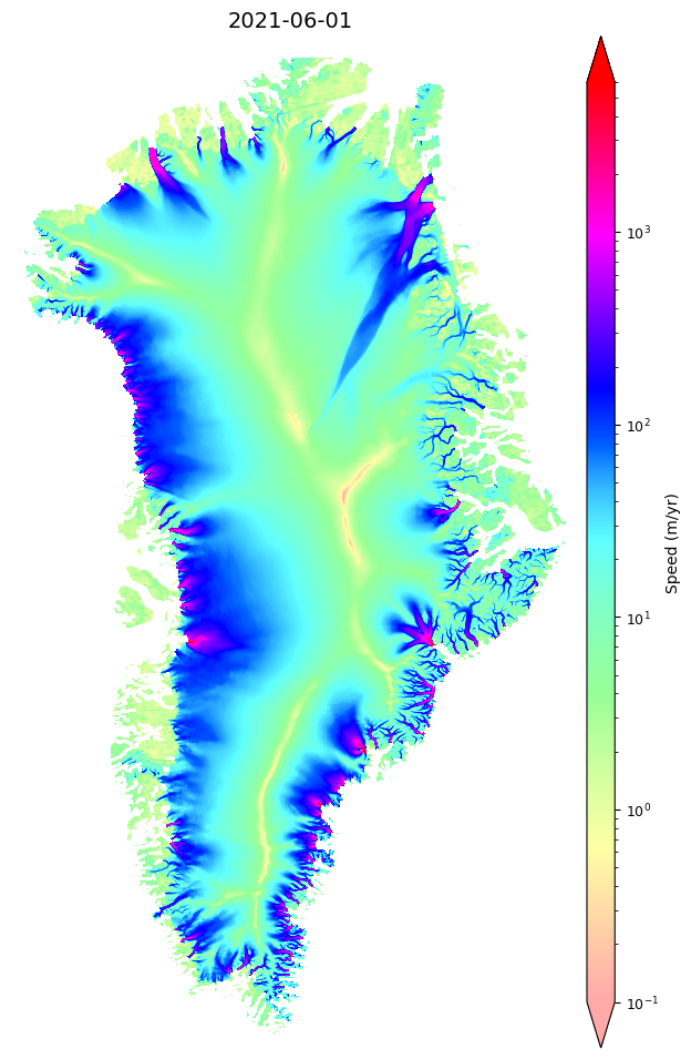
time2 datetime64[ns] 2021-11-30✅ Examining interesting velocity map features#
We can use the:
myVelSeries = nisar.nisarVelSeries.displayVelForDate()
function to plot the velocity map for the annual mosaic nearest the user-provided date ⬇.
myVelSeries.displayVelForDate('2021-06-01',labelFontSize=10, plotFontSize=9, titleFontSize=14,
                              vmin=0, vmax=6000,scale='log',colorBarPad=0.15,units='km', axisOff=True)
[########################################] | 100% Completed | 343.68 ms
[########################################] | 100% Completed | 101.74 ms
<matplotlib.image.AxesImage at 0x7fbae8d25fc0>
🚨 These files can be large!#
Below are functions that allow you to quickly subset the data by spatial bounds, including the functions you can use to interactively select an ROI when exploring datasets remotely
Method 1: Interactive ROI Selection#
Run the next the tool below to select the bounding box (or modify a manually selected box), which will display a SAR image map. Depending on network speed, it could take a few seconds to a minute to load the basemap. Use the box tool in the plot menu to select a region of interest.
Interactive ROI selection
Paste the code below in a new cell to try interactive bounding box selection
: if ‘boxPicker’ not in locals(): # Only create if not defined above boxPicker = grimp.boxPicker() boxPicker.plotMap(show=(not myUrls.checkIDs([‘NSIDC-0481’]) and not myUrls.checkIDs([‘NSIDC-0646’])))
Method 2: Manual Selection#
The coordinates for bounding box, bbox, can be manually entered by modifying the cell below with the desired values. Even if not using interactive selection, running that step displays the manually selected box coordinates on a radar map of Greenland. Note by default, coordinates are rounded to the nearest kilometer. We will use a predefined bbox for the tutorial today.
values = np.around([-472889, -2540695, -453487, -2523127])
xyBounds = dict(zip(['minx', 'miny', 'maxx', 'maxy'], values))
xyBounds

myVelSeries.subSetVel(xyBounds)
myVelSeries.subset
<xarray.DataArray 'VelocitySeries' (time: 1, band: 3, y: 22, x: 25)>
dask.array<getitem, shape=(1, 3, 22, 25), dtype=float32, chunksize=(1, 1, 22, 25), chunktype=numpy.ndarray>
Coordinates:
  * band         (band) <U2 'vx' 'vy' 'vv'
  * x            (x) float64 -4.731e+05 -4.723e+05 ... -4.547e+05 -4.539e+05
  * y            (y) float64 -2.524e+06 -2.524e+06 ... -2.54e+06 -2.54e+06
  * time         (time) datetime64[ns] 2021-06-01
    name         <U4 'None'
    _FillValue   (band) float64 -2e+09 -2e+09 -1.0
    time1        datetime64[ns] 2020-12-01
    time2        datetime64[ns] 2021-11-30
spatial_ref int64 0The data in the above example map are stored as an Xarray, velMap.subset. In this case, the subset is the full map of Greenland for one time slice. The full time series of Greenland-wide mosiacs can reach sizes of > 8GB and may take awhile to download! Because of the lazy open mentioned above, the data have not been downloaded or read from the disk yet. Before applying the final subset, its useful to examine the size of the full data (virtual) array. If the loadDataArray step was successful, this next cell will provide details on the size and organization of the full xarray (prior to any download).
Optionally download subset as netcdf file
The downloaded subset can be saved in a netcdf and reloaded for to velSeries instance for later analysis. Note if the data have been subsetted, ONLY the subset will be saved - so it is not a bad idea to check out the dimensions, variable names, and total size of the subset data one last time prior to downloading.
: Add comment on xy bounds
: myVelSeries.subSetVel(xyBounds)
myVelSeries.subset
: Add comment on export to cdf : subsetFile = ‘steenstrupGlacier_annVel.nc’ myVelSeries.loadRemote() myVelSeries.toNetCDF(subsetFile)
For today, however, we are going to assume we have already subset and downloaded our area and variable of interest, and read in velocities over Steenstrup Glacier, Greenland.#
# Now reload the downloaded data
myVelReload = nisar.nisarVelSeries()
myVelReload.readSeriesFromNetCDF('./res/steenstrupGlacier_annVel.nc')
myVelReload.loadRemote()
myVelReload.xr #confirm dimensions of read-in subsetted velocities
<xarray.DataArray 'VelocitySeries' (time: 7, band: 3, y: 351, x: 306)>
array([[[[ 1.11676419e+00,  1.59998286e+00,  1.70799983e+00, ...,
           2.30640930e+02,  1.47605362e+02,  6.85445480e+01],
         [ 6.27350628e-01,  1.19134200e+00,  1.44590247e+00, ...,
           2.89960114e+02,  2.18558105e+02,  1.22185051e+02],
         [-1.73795328e-01,  1.81840569e-01,  1.62274435e-01, ...,
           3.05869354e+02,  2.55354233e+02,  1.62863892e+02],
         ...,
         [-4.73510027e+00, -5.52709627e+00, -5.25623894e+00, ...,
                      nan,             nan,             nan],
         [-2.86730933e+00, -3.33576107e+00, -3.83880162e+00, ...,
                      nan,             nan,             nan],
         [-1.34066474e+00, -1.90317583e+00, -2.72140670e+00, ...,
                      nan,             nan,             nan]],

        [[-5.82537270e+00, -5.66549730e+00, -5.22123241e+00, ...,
          -1.92974136e+02, -1.38507278e+02, -8.94227600e+01],
         [-4.98156023e+00, -4.58929014e+00, -3.94673991e+00, ...,
          -2.78241943e+02, -2.42269043e+02, -1.87016388e+02],
         [-4.90611362e+00, -4.50508499e+00, -3.54733062e+00, ...,
          -3.45336029e+02, -3.39918884e+02, -2.98722015e+02],
...
                      nan,             nan,             nan],
         [ 2.78865981e+00,  3.08081293e+00,  4.41497707e+00, ...,
                      nan,             nan,             nan],
         [ 6.93372369e-01,  2.12009978e+00,  3.43272281e+00, ...,
                      nan,             nan,             nan]],

        [[ 1.84553146e+00,  1.68653011e+00,  1.81761539e+00, ...,
           3.44428375e+02,  2.52386292e+02,  1.46040314e+02],
         [ 2.93052220e+00,  2.40399122e+00,  1.62190270e+00, ...,
           4.64432281e+02,  3.87946686e+02,  2.72755463e+02],
         [ 3.41516590e+00,  3.03598475e+00,  2.22783017e+00, ...,
           5.79738403e+02,  5.25995850e+02,  4.15923523e+02],
         ...,
         [ 6.43459558e+00,  7.29936552e+00,  7.30895853e+00, ...,
                      nan,             nan,             nan],
         [ 3.84925318e+00,  4.81166029e+00,  5.59751654e+00, ...,
                      nan,             nan,             nan],
         [ 3.06430936e+00,  3.67955160e+00,  4.11497211e+00, ...,
                      nan,             nan,             nan]]]],
      dtype=float32)
Coordinates:
    _FillValue   float64 -1.0
  * time         (time) datetime64[ns] 2015-06-01 ... 2021-06-01
    id           (time) object 'https://n5eil01u.ecs.nsidc.org/DP4/MEASURES/N...
  * band         (band) object 'vx' 'vy' 'vv'
  * x            (x) float64 4.19e+05 4.192e+05 4.194e+05 ... 4.798e+05 4.8e+05
  * y            (y) float64 -2.486e+06 -2.486e+06 ... -2.556e+06 -2.556e+06
    epsg         int64 3413
    name         <U4 'temp'
    time1        (time) datetime64[ns] 2014-12-01 2015-12-01 ... 2020-12-01
    time2        (time) datetime64[ns] 2015-11-30 2016-11-30 ... 2021-11-30
    spatial_ref  int64 0
Attributes: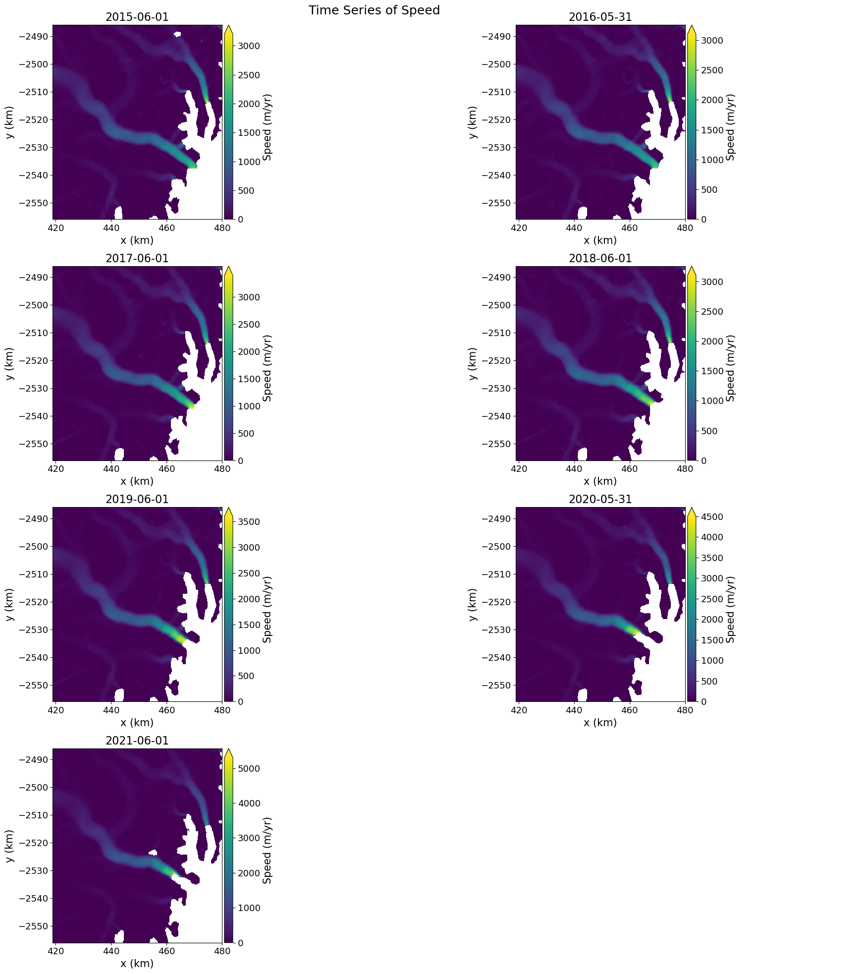
grid_mapping: spatial_refWe can plot the annual velocity maps for Steenstrup Glacier.#
fig, axes = plt.subplots(4, 2,figsize=(20,20))

for ax, date in zip(axes.flatten(), myVelReload.time):
    myVelReload.displayVelForDate(date=date, ax=ax,units='km')
axes[-1, -1].axis('off'); #remove any empty axes if odd number of years
fig.suptitle('Time Series of Speed', fontsize=18)
fig.tight_layout()
📈 Explore multiyear trends using the interactive inspection tool in the cell block below ⬇#
myVelReload.inspect()
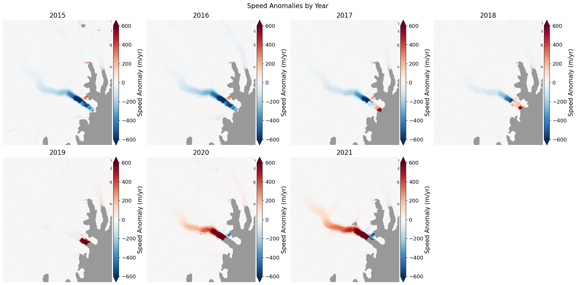
📊 Quickly plot velocity anomalies#
computes [velocity at t_i - mean] of all timesteps in data series
velAnomaly = myVelReload.anomaly()

# Plot the anomaly for each year
fig, axes = plt.subplots(2, 4, figsize=(20,10))
for date, ax in zip(velAnomaly.time, axes.flatten()):
    velAnomaly.displayVelForDate(date, ax=ax, units='m', vmin=-600, vmax=600, autoScale=False, axisOff=True,
                                 title=date.strftime("%Y"),cmap='RdBu_r', colorBarLabel='Speed Anomaly (m/yr)',
                                 extend='both',backgroundColor=(0.6, 0.6, 0.6))
axes[-1, -1].axis('off'); # kill axis with no plot
fig.suptitle('Speed Anomalies by Year', fontsize=16)
fig.tight_layout()
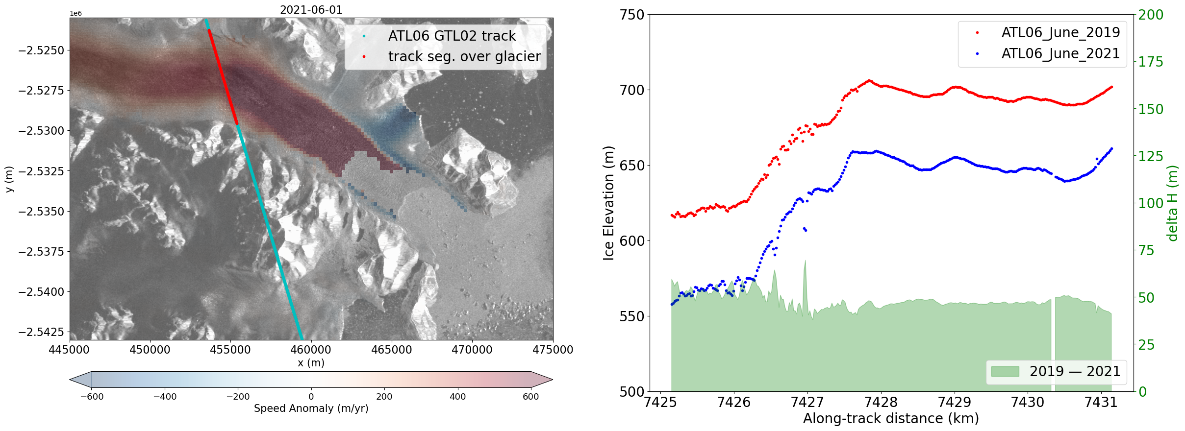
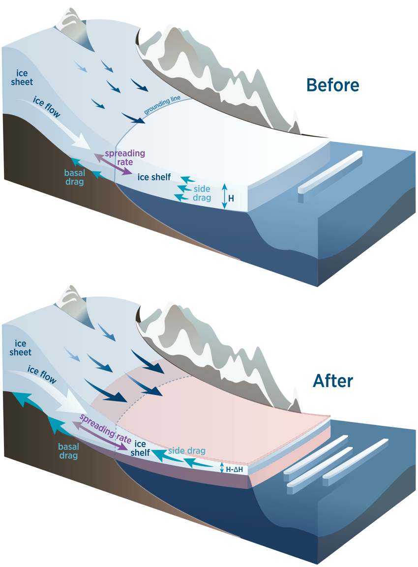
Dynamic Thinning at ice sheet margins#
Typically, we expect a rapid acceleration in ice flow to also correspond with dynamic ice thinning. Let’s use ICESat-2 data to see if that is true for Steenstrup Glacier.
Accessing from the cloud (outside of tutorial)
Follow the example block of code below to access non-local data outside of tutorial
: Give ROI, product, and temporal range to query using icepyx : spatial_extent = [-34.8799,66.4665,-34.3847,66.6506] region_a = ipx.Query(‘ATL06’,spatial_extent,[‘2019-01-01’,’2021-12-31’]) region_a.earthdata_login()
: Explore variables, select those of interest and download submitted granule order. : region_a.show_custom_options(dictview=True) region_a.order_vars.avail(options=True) region_a.visualize_spatial_extent() region_a.download_granules(‘/home/jovyan/icesat2data’) #download path (replace with preferred directory)
Use Ben Smith’s function to read in ATL06 (ICESat-2 land ice product) data from local files#
def atl06_to_dict(filename, beam, field_dict=None, index=None, epsg=None):
    """
        Read selected datasets from an ATL06 file

        Input arguments:
            filename: ATl06 file to read
            beam: a string specifying which beam is to be read (ex: gt1l, gt1r, gt2l, etc)
            field_dict: A dictionary describing the fields to be read
                    keys give the group names to be read,
                    entries are lists of datasets within the groups
            index: which entries in each field to read
            epsg: an EPSG code specifying a projection (see www.epsg.org).  Good choices are:
                for Greenland, 3413 (polar stereographic projection, with Greenland along the Y axis)
                for Antarctica, 3031 (polar stereographic projection, centered on the Pouth Pole)
        Output argument:
            D6: dictionary containing ATL06 data.  Each dataset in
                dataset_dict has its own entry in D6.  Each dataset
                in D6 contains a numpy array containing the
                data
    """
    if field_dict is None:
        field_dict={None:['latitude','longitude','h_li', 'atl06_quality_summary'],\
                    'ground_track':['x_atc','y_atc'],\
                    'fit_statistics':['dh_fit_dx', 'dh_fit_dy']}
    D={}
    file_re=re.compile('ATL06_(?P<date>\d+)_(?P<rgt>\d\d\d\d)(?P<cycle>\d\d)(?P<region>\d\d)_(?P<release>\d\d\d)_(?P<version>\d\d).h5')
    with h5py.File(filename,'r') as h5f:
        for key in field_dict:
            for ds in field_dict[key]:
                if key is not None:
                    ds_name=beam+'/land_ice_segments/'+key+'/'+ds
                else:
                    ds_name=beam+'/land_ice_segments/'+ds
                if index is not None:
                    D[ds]=np.array(h5f[ds_name][index])
                else:
                    D[ds]=np.array(h5f[ds_name])
                if '_FillValue' in h5f[ds_name].attrs:
                    bad_vals=D[ds]==h5f[ds_name].attrs['_FillValue']
                    D[ds]=D[ds].astype(float)
                    D[ds][bad_vals]=np.NaN
    if epsg is not None:
        xy=np.array(pyproj.proj.Proj(epsg)(D['longitude'], D['latitude']))
        D['x']=xy[0,:].reshape(D['latitude'].shape)
        D['y']=xy[1,:].reshape(D['latitude'].shape)
    temp=file_re.search(filename)
    D['rgt']=int(temp['rgt'])
    D['cycle']=int(temp['cycle'])
    D['beam']=beam
    return D
# Read in local SAR mosaic of our glacier of interest
img_name = '/home/jovyan/shared-public/GeoTIFF/GL_S1bks_mosaic_uncalibrated._2021-08-05.tif'
img = rasterio.open(img_name)

# read in first band of imagery
array = img.read(1)
array[array < 0] = 0

# Read ATL06 land ice elevation from GT2l track
ATL06_file0=('./res/processed_ATL06_20191106230008_06270503_006_01.h5')
D0=atl06_to_dict(ATL06_file0,'/gt2l', index=None, epsg=3413)
ATL06_file1=('./res/processed_ATL06_20211102121853_06271303_006_01.h5')
D1=atl06_to_dict(ATL06_file1,'/gt2l', index=None, epsg=3413)
Now plot ICESat-2 and velocity change together to evaluate if dynamic thinning occurred#
fig = plt.figure(figsize=(28,10))
ax1 = plt.subplot(1,2,1)
ax2 = plt.subplot(1,2,2)

#ax1
bounds = np.linspace(-15, 210, 255)
norm = mcolors.BoundaryNorm(boundaries=bounds, ncolors=256, extend='both')
rasterio.plot.show(array,ax=ax1,cmap='gist_gray',transform=img.transform,norm=norm)
velAnomaly.displayVelForDate('2021-06-01', ax=ax1, units='m', vmin=-600, vmax=600, autoScale=False,colorBarPosition='bottom',
                        colorBarPad=0.65,colorBarSize='5%',cmap='RdBu_r', colorBarLabel='Speed Anomaly (m/yr)',
                        extend='both',alpha=0.3)

ax1.plot(D1['x'], D1['y'],'c.',label='ATL06 GTL02 track')
ax1.plot(D1['x'][700:1000], D1['y'][700:1000],'r.',label='track seg. over glacier')
ax1.set_xlim(445000,475000)
ax1.set_ylim(-2543000,-2523000)
ax1.legend(fontsize=20);
ax1.tick_params(axis='both', labelsize=16)

#ax2
ax2.plot(0.001*D0['x_atc'][700:1000], D0['h_li'][700:1000],'r.', label='ATL06_June_2019')
ax2.plot(0.001*D1['x_atc'][700:1000], D1['h_li'][700:1000],'b.', label='ATL06_June_2021')
ax2.set_ylim(500,750)
ax2.tick_params(axis='both', labelsize=20)
ax2.set_ylabel('Ice Elevation (m)',fontsize=20)
ax2.set_xlabel('Along-track distance (km)',fontsize=20)
ax2.legend(fontsize=20);

#calculate 2019 - 2021 difference in elevation
ax_c = ax2.twinx()

deltaH = D0['h_li'][700:1000]- D1['h_li'][700:1000]
deltaH[deltaH > 200] = np.NaN

ax_c.fill_between(0.001*D0['x_atc'][700:1000],deltaH,color='green',alpha=0.3,label='2019 — 2021')
ax_c.set_ylim(0,200)
ax_c.tick_params(axis='y', labelsize=20,labelcolor='green',color='green')
ax_c.set_ylabel('delta H (m)',fontsize=20,color='green');
ax_c.legend(loc='lower right',fontsize=20);