ICESat-2 sea ice tutorial

⭐ Objectives

• Learn how to access/download ICESat-2 sea ice products (ATL07/ATL10/ATL20) via icepyx or earthaccess libraries.

• Examine what the ICESat-2 sea ice freeboard products (ATL10/ATL20) look like.

• Derive sea ice properties (sea ice thickness, floe size distribution, lead fraction) using ATL10 product.

• Map monthly sea ice freeboard using ATL20 product.

📌 What is sea ice?

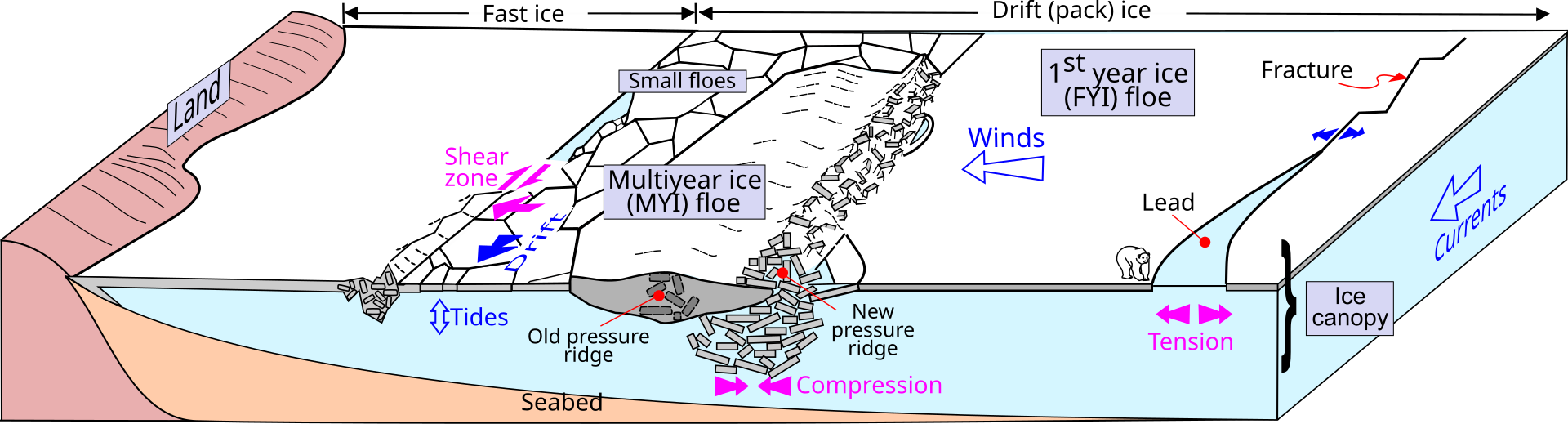
Fig. 1 Schematic diagram of common sea-ice related features.

Sea ice is frozen seawater that floats on the ocean surface. It forms in both the Arctic and the Antarctic in each hemisphere’s winter; it retreats in the summer, but does not completely disappear. Sea ice is not just a “flat” surface. Sea ice surface is very dynamic, so sea ice surface consists of various topograhic features, such as ridges (occur when sea ice floes collide) or leads (open water or thin ice space between sea ice floes). The fine resolution of ICESat-2 allows us to detect the details of these sea ice dynamic features.

📌 How can laser altimeters measure sea ice freeboard/thickness?

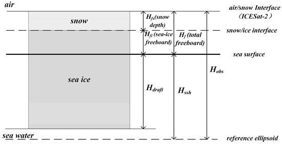
Fig. 2 Schematic diagram of sea ice height and sea ice freeboard (source: Pang et al. 2022)

Sea ice freeboard means the height of sea ice surface above local sea surface. To calculate sea ice freeboard, it is necessary to subtract local sea surface height from the sea ice height.

\(H_{f} = H_{obs} - H_{ssh}\)

The ATL07 product provides the surface height above the reference ellipsoid (WGS84). The ATL07 product aggregates 150 signal photons as a single “height segment”, and the mean height of this segment is determined as the surface height. In general, each height segment has 10-20 m of length (strong beams).

Then, in order to calculate sea ice freeboard, it is necessary to separate the height signal from open water (lead) and sea ice surface. The ATL07 product has its own algorithm to distinguish leads from sea ice. There are two types of leads detected by the ATL07: specular lead (high photon rate/reflectance) and dark lead (low photon rate/reflectance).

Fig. 3 Example of ATL07 profile and surface classification with overlapped optical image (source: Petty et al. 2022)

The ATL10 product calculates the height difference between sea ice surface and lead surface. The local sea level (\(H_{ssh}\)) is calculated for every 10 km using detected leads.

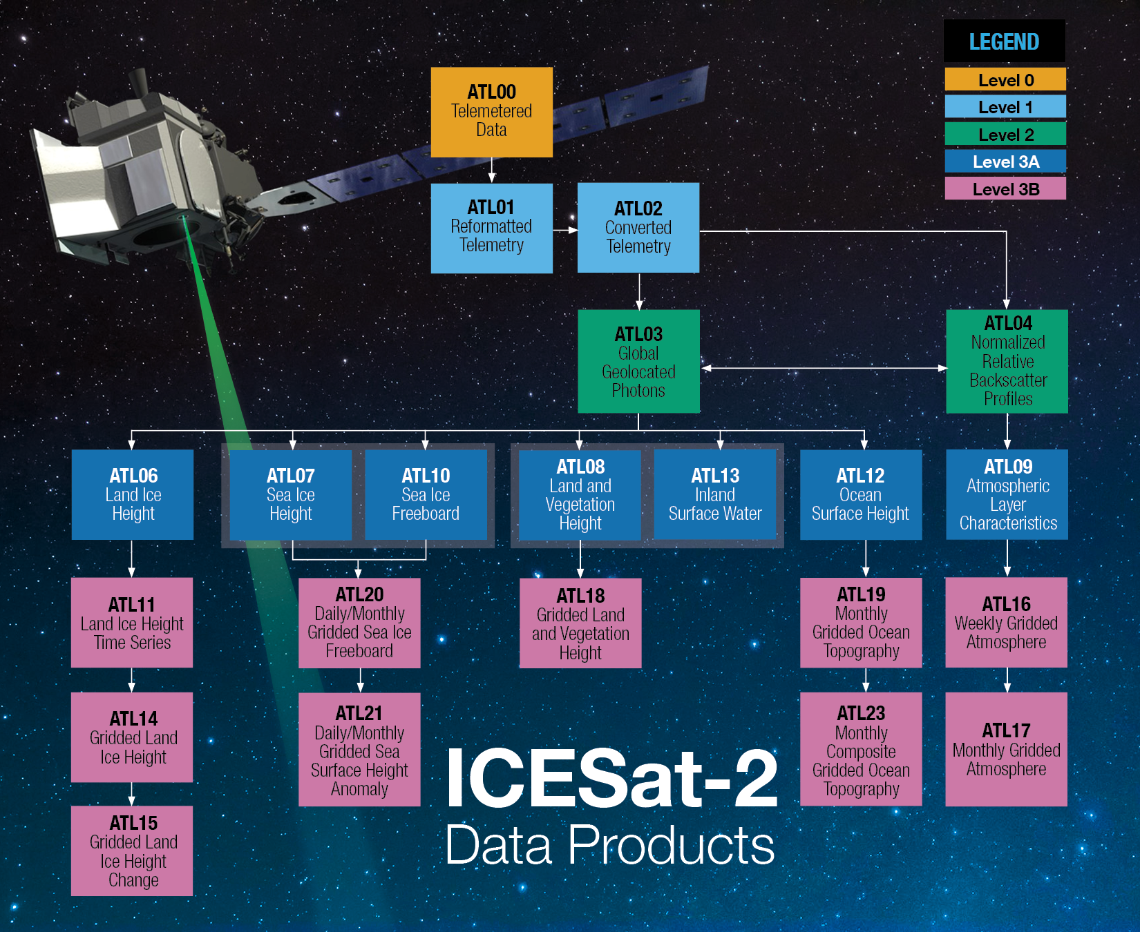
📌 ICESat-2 sea ice products

• ATL07 (sea ice surface heights): Surface height relative to WGS84 ellipsoid. Derived by aggregating 150 signal photons of the ATL03 product.

• ATL10 (freeboard): Sea ice freeboard calculated from ATL07 product.

• ATL20 (daily/monthly gridded sea ice freeboard): 25-km gridded mean freeboard in daily/monthly scale.

Fig. 4 ICESat-2 products (source: NSIDC)

✅ Access & Download sea ice products (1) - Use icepyx

In this tutorial, first, we will use icepyx library to access or download ICESat-2 datasets.

import warnings
warnings.filterwarnings('ignore')

import icepyx as ipx
import earthaccess

After importing icepyx library, we will create an query to request ICESat-2 data for our region/time of interest.

# Data product: ATL10 (sea ice freeboard)
short_name = 'ATL10'

# Spatial extent: Ross Sea, Antarctica
spatial_extent = [-180, -78, -160, -74]

# Time range
date_range = ['2019-09-16','2019-09-16'] # first time period
# date_range = ['2019-11-13','2019-11-13'] # second time period

reg=ipx.Query(short_name, spatial_extent, date_range,
              start_time = "12:00:00", endtime = "20:00:00")

# Visualize the spatial extent
reg.visualize_spatial_extent()

/srv/conda/envs/notebook/lib/python3.10/site-packages/geoviews/operation/__init__.py:14: HoloviewsDeprecationWarning: 'ResamplingOperation' is deprecated and will be removed in version 1.18, use 'ResampleOperation2D' instead.
  from holoviews.operation.datashader import (

print(reg.latest_version())
reg.product_summary_info()

006
title :  ATLAS/ICESat-2 L3A Sea Ice Freeboard V006
short_name :  ATL10
version_id :  006
time_start :  2018-10-14T00:00:00.000Z
coordinate_system :  CARTESIAN
summary :  This data set (ATL10) contains estimates of sea ice freeboard, calculated using three different approaches. Sea ice leads used to establish the reference sea surface and descriptive statistics used in the height estimates are also provided. The data were acquired by the Advanced Topographic Laser Altimeter System (ATLAS) instrument on board the Ice, Cloud and land Elevation Satellite-2 (ICESat-2) observatory.
orbit_parameters :  {'swath_width': '36.0', 'period': '96.8', 'inclination_angle': '92.0', 'number_of_orbits': '1.0', 'start_circular_latitude': '0.0'}

(i) Open an ICESat-2 granule directly from the S3 bucket

You can remotely access the ICESat-2 data stored in the S3 bucket.

# Earthdata login information: Please put your own account information
reg.earthdata_login(s3token=True)

EARTHDATA_USERNAME and EARTHDATA_PASSWORD are not set in the current environment, try setting them or use a different strategy (netrc, interactive)
No .netrc found in /home/jovyan

Enter your Earthdata Login username:  younghyunkoo
Enter your Earthdata password:  ········

You're now authenticated with NASA Earthdata Login
Using token with expiration date: 09/11/2023
Using user provided credentials for EDL

s3links = reg.avail_granules(cloud=True)[0]  # returns a nested list, get first element
s3links

['s3://nsidc-cumulus-prod-protected/ATLAS/ATL10/006/2019/09/16/ATL10-02_20190916205836_12340401_006_02.h5']

(ii) Local download

Otherwise, if you want to download these files into your local computer, you can use the below scripts.

reg.earthdata_login()

# Check the granule ids
gran_ids = reg.avail_granules(ids=True)[0]
gran_ids

# Order granules
reg.order_granules()

# Download granules
path = "" # you can put your own directory where you want to download the files.
reg.download_granules(path)

✅ Access & Download sea ice products (2) - Use Earthaccess

There is another way to access ICESat-2 data using another Python library Earthaccess. In the following Earthaccess example, you can access the raw ICESat-2 data remotely without downloading them to your local machine.

auth = earthaccess.login()

We are already authenticated with NASA EDL

Query = earthaccess.collection_query().keyword('ICESat-2')

Query.hits()

69

Query = earthaccess.collection_query().keyword('ATL10').cloud_hosted(True)
print(Query.hits())
collections = Query.fields(['ShortName', 'Version']).get(25)
print(collections)

4
[{
  "meta": {
    "concept-id": "C2613553243-NSIDC_CPRD",
    "granule-count": 39957,
    "provider-id": "NSIDC_CPRD"
  },
  "umm": {
    "ShortName": "ATL10",
    "Version": "006"
  }
}, {
  "meta": {
    "concept-id": "C2153574813-NSIDC_CPRD",
    "granule-count": 35693,
    "provider-id": "NSIDC_CPRD"
  },
  "umm": {
    "ShortName": "ATL10",
    "Version": "005"
  }
}, {
  "meta": {
    "concept-id": "C2153577387-NSIDC_CPRD",
    "granule-count": 96,
    "provider-id": "NSIDC_CPRD"
  },
  "umm": {
    "ShortName": "ATL20",
    "Version": "003"
  }
}, {
  "meta": {
    "concept-id": "C2153577500-NSIDC_CPRD",
    "granule-count": 96,
    "provider-id": "NSIDC_CPRD"
  },
  "umm": {
    "ShortName": "ATL21",
    "Version": "002"
  }
}]

Query = earthaccess.granule_query().concept_id(
    'C2153574813-NSIDC_CPRD'
).temporal("2019-11-13 T10:00:00", "2019-11-13 T20:00:00"
).bounding_box(-180, -77, -160, -74)

# Bounding box: [West lon, South lat, East lon, North lat]
# ATL07: C2153574585-NSIDC_CPRD
# ATL10: C2153574813-NSIDC_CPRD
# ATL20: C2153577387-NSIDC_CPRD

Query.hits()

1

granules = Query.get(1)
[display(g) for g in granules];

Data: ATL10-02_20191113181045_07310501_005_02.h5

Size: 151.16 MB

Cloud Hosted: True

files = earthaccess.open(granules)
files

 Opening 1 granules, approx size: 0.15 GB

[<File-like object S3FileSystem, nsidc-cumulus-prod-protected/ATLAS/ATL10/005/2019/11/13/ATL10-02_20191113181045_07310501_005_02.h5>]

✅ Explore ATL10 sea ice freeboard product (single track)

Now, we will explore what the ATL10 sea ice freeboard data really looks like. Let’s start with the two example tracks in the Ross Sea, Antarctica.

Import necessary libraries

import h5py
import pyproj

# Ignore warning
import warnings
warnings.filterwarnings("ignore")

import cartopy.crs as ccrs

%matplotlib widget
import matplotlib.pyplot as plt

import numpy as np
import pandas as pd

Read first track

Read local downloaded files

## IF you want to access local downloaded files, please use the below codes.
# H5 file of the ATL10 track
tutorial_data = "/home/jovyan/shared-public/ICESat-2-Hackweek/sea_ice"
filename = f"{tutorial_data}/processed_ATL10-02_20190916205836_12340401_006_02.h5"
filename

Read cloud files

## IF you want to access the file via S3 bucket, please use the below codes.
s3 = earthaccess.get_s3fs_session(daac='NSIDC')
filename = s3.open(s3links[0], 'rb')
filename

<File-like object S3FileSystem, nsidc-cumulus-prod-protected/ATLAS/ATL10/006/2019/09/16/ATL10-02_20190916205836_12340401_006_02.h5>

# Check the orbit orientation
with h5py.File(filename,'r') as f:
    orient = f['orbit_info/sc_orient'][0]

# 0: backward; 1: forward; 2: transition (do not use)
print(orient)

1

🔍 Which beam is strong/weak?

The relative location of strong and beak beams depends on the orientation of the satellite orbit. If the satellite moves in forward direction, right beams (i.e., GT1R, GT2R, GT3R) are STRONG beams. On the contrary, in the case of backward direction, left beams (i.e., GT1L, GT2L, GT3L) are WEAK beams.

Fig. 5 Orbit orientation and strong/weak beam of ICESat-2 (source: Kwok et al. 2019)

## Function to read ATL10 data
def read_atl10(filename, spatial_extent):

    # Create a list for saving ATL10 beam track data
    track = []

    with h5py.File(filename,'r') as f:

        # Check the orbit orientation
        orient = f['orbit_info/sc_orient'][0]

        if orient == 0:
            strong_beams = [f"gt{i}l" for i in [1, 2, 3]]
        elif orient == 1:
            strong_beams = [f"gt{i}r" for i in [1, 2, 3]]
        else:
            strong_beams = []

        for beam in strong_beams:

            lat = f[beam]['freeboard_segment/latitude'][:]
            lon = f[beam]['freeboard_segment/longitude'][:]
            seg_x = f[beam]['freeboard_segment/seg_dist_x'][:] / 1000 # (m to km)
            seg_len = f[beam]['freeboard_segment/heights/height_segment_length_seg'][:]
            fb = f[beam]['freeboard_segment/beam_fb_height'][:]
            surface_type = f[beam]['freeboard_segment/heights/height_segment_type'][:]
            fb[fb>100] = np.nan

            df = pd.DataFrame({'lat': lat, 'lon': lon, 'seg_x': seg_x, 'seg_len': seg_len,
                              'freeboard': fb, 'stype': surface_type})

            df = df[(df['lat'] > spatial_extent[1]) & (df['lat'] < spatial_extent[3])].reset_index(drop=True)

            df['beam'] = beam
            df = df.dropna().reset_index(drop = True)

            track.append(df)
            
    return track

track = read_atl10(filename, spatial_extent)

Draw freeboard track

# Select which beam you want to explore (0, 1, 2)
df = track[0]

plt.figure(figsize = (8, 3))

# Masking for normal sea ice
mask_ice = (df.stype == 1)

# Masking for specular lead
mask_specular = (df.stype >= 2) & (df.stype <= 5)

# Masking for dark lead
mask_dark = (df.stype >= 6) & (df.stype <= 9)

plt.scatter(df.seg_x[mask_ice], df.freeboard[mask_ice], s = 2, color = "c", label = "Non-lead")
plt.scatter(df.seg_x[mask_specular], df.freeboard[mask_specular], s = 5, color = "r", label = "Specular lead")
plt.scatter(df.seg_x[mask_dark], df.freeboard[mask_dark], s = 5, color = "k", label = "Dark lead")
plt.axhline(0.15, color = "b", ls = "--")
plt.xlabel("Along-track distance (km)")
plt.ylabel("Freeboard (m)")
plt.legend()

# plt.xlim(32890, 32920)
plt.tight_layout()

## Calculate lead fraction
print("Sea ice (%): ", np.sum(df.seg_len[mask_ice]) / np.sum(df.seg_len) * 100)
print("Specular lead (%): ", np.sum(df.seg_len[mask_specular]) / np.sum(df.seg_len) * 100)
print("Dark lead (%): ", np.sum(df.seg_len[mask_dark]) / np.sum(df.seg_len) * 100)
print("Freeboard < 0.1 m (%): ", np.sum(df.seg_len[df.freeboard < 0.1]) / np.sum(df.seg_len) * 100)

Sea ice (%):  97.82050251960754
Specular lead (%):  0.16137033235281706
Dark lead (%):  2.018122561275959
Freeboard < 0.15 m (%):  6.698114424943924

Draw freeboard histograms

plt.figure(figsize = (8, 4))
for df in track:
    
    plt.hist(df['freeboard'], bins = 100, range = (0,2), label = df.beam[0], histtype = 'step')
    print(f"Beam {df.beam[0]}")
    print(f"   - mean freeboard: {df.freeboard.mean():.3f} m")
    print(f"   - std. dev. freeboard: {df.freeboard.std():.3f} m")
    
plt.xticks(np.arange(0,2,0.1))
plt.xlim(0,2)
plt.grid(ls = ":", lw = 0.5)
plt.legend()
plt.xlabel("Freeboard (m)")
plt.ylabel("Count")
plt.show()

Beam gt1r
   - mean freeboard: 0.504 m
   - std. dev. freeboard: 0.360 m
Beam gt2r
   - mean freeboard: 0.515 m
   - std. dev. freeboard: 0.387 m
Beam gt3r
   - mean freeboard: 0.506 m
   - std. dev. freeboard: 0.396 m

💡 Do it yourself!

Let’s try the same steps for another track data for the Ross Sea Sea region. The first track we just examined is from September, but this second track is from November. Compare how the freeboard and lead fraction has been changed for these two months.

tutorial_data = "/home/jovyan/shared-public/ICESat-2-Hackweek/sea_ice"
filename = f"{tutorial_data}/processed_ATL10-02_20191113181045_07310501_006_01.h5"

# Plot lead fraction, floe size distribution, mean freeboard, etc.

✅ Explore sea ice freeboard products (gridded product)

Now we will explore gridded sea ice freeboard product (ATL20).

Antarctic example

We will visualize the Antractic sea ice in September 2021. In general, the Antarctic sea ice extent reaches maximum in September, so you will be able to see the maximum sea ice extent.

# Query Antarctic ATL20 data using earthaccess (September)
Query = earthaccess.granule_query().concept_id(
    'C2153577387-NSIDC_CPRD'
).temporal("2021-09-01 T10:00:00", "2021-09-30 T23:00:00"
).bounding_box(-180, -90, 180, -60)

granules = Query.get()
granules

[Collection: {'EntryTitle': 'ATLAS/ICESat-2 L3B Daily and Monthly Gridded Sea Ice Freeboard V003'}
 Spatial coverage: {'HorizontalSpatialDomain': {'Geometry': {'BoundingRectangles': [{'WestBoundingCoordinate': -179.999992, 'EastBoundingCoordinate': 179.999999, 'NorthBoundingCoordinate': -53.516075, 'SouthBoundingCoordinate': -78.481569}]}}}
 Temporal coverage: {'RangeDateTime': {'BeginningDateTime': '2021-09-01T01:52:44.289Z', 'EndingDateTime': '2021-10-01T00:18:47.822Z'}}
 Size(MB): 2.6486663818359375
 Data: ['https://data.nsidc.earthdatacloud.nasa.gov/nsidc-cumulus-prod-protected/ATLAS/ATL20/003/2021/ATL20-02_20210901005050_10601201_003_01.h5']]

# Open file
files = earthaccess.open(granules)
files[0]

 Opening 1 granules, approx size: 0.0 GB

<File-like object S3FileSystem, nsidc-cumulus-prod-protected/ATLAS/ATL20/003/2021/ATL20-02_20210901005050_10601201_003_01.h5>

# Read h5 file
with h5py.File(files[0],'r') as f:
    mean_fb = f['monthly']['mean_fb'][:]
    mean_fb[mean_fb > 1000] = np.nan
    
    # ATL20 is 25 km grid data
    lat = f['grid_lat'][:] # Latitude
    lon = f['grid_lon'][:] # Longitude
    
    # Spatial reference: NSIDC Sea Ice Polar Stereographic South (EPSG:3412)
    x = f['grid_x'][:]
    y = f['grid_y'][:]
    xx, yy = np.meshgrid(x, y)

fig=plt.figure(figsize=(6, 6))

# Use the in-built northpolarstereo to visualize (true scale latitude is from NSIDC polar stereographic)
ax = plt.axes(projection = ccrs.SouthPolarStereo(central_longitude=0, true_scale_latitude = -70))

pm  = ax.pcolormesh(xx ,yy, mean_fb, vmin = 0, vmax = 0.8)
ax.coastlines('10m', linewidth = 0.5) # add coastline
# Add gridline
gl = ax.gridlines(crs=ccrs.PlateCarree(), draw_labels=True,
                  linewidth=1, color='lightgrey', alpha=0.5, linestyle='--')

clb = plt.colorbar(pm, ax = ax, shrink = 0.4)
clb.set_label('Sea ice freeboard (m)', rotation = 270, fontsize = 11, va = 'bottom')
plt.show()

Arctic example

For the Arctic, we will visualize sea ice freeboard map in March 2021.

Query = earthaccess.granule_query().concept_id(
    'C2153577387-NSIDC_CPRD'
).temporal("2021-03-01 T10:00:00", "2021-03-30 T23:00:00"
).bounding_box(-180, 60, 180, 90)

granules = Query.get()

files = earthaccess.open(granules)

with h5py.File(files[0],'r') as f:
    mean_fb = f['monthly']['mean_fb'][:]
    mean_fb[mean_fb > 1000] = np.nan

    lat = f['grid_lat'][:]
    lon = f['grid_lon'][:]
    
    # Spatial reference: NSIDC Sea Ice Polar Stereographic North (EPSG:3411)
    x = f['grid_x'][:]
    y = f['grid_y'][:]
    xx, yy = np.meshgrid(x, y)

 Opening 1 granules, approx size: 0.0 GB

fig=plt.figure(figsize=(6, 6))
# Use the in-built northpolarstereo to visualize (true scale latitude is from NSIDC polar stereographic)
ax = plt.axes(projection = ccrs.NorthPolarStereo(central_longitude=-45, true_scale_latitude = 70))

pm  = ax.pcolormesh(xx ,yy, mean_fb, vmin = 0, vmax = 0.8)
ax.coastlines('10m', linewidth = 0.5)

gl = ax.gridlines(crs=ccrs.PlateCarree(), draw_labels=True,
                  linewidth=1, color='lightgrey', alpha=0.5, linestyle='--')
clb = plt.colorbar(pm, ax = ax, shrink = 0.4)
clb.set_label('Sea ice freeboard (m)', rotation = 270, fontsize = 11, va = 'bottom')

💡 Do it yourself!

Let’s visualize the griddged freeboard for another month.

Helpful references

• Kwok, R., Markus, T., Kurtz, N. T., Petty, A. A., Neumann, T. A., Farrell, S. L., et al. (2019). Surface height and sea ice freeboard of the Arctic Ocean from ICESat-2: Characteristics and early results. Journal of Geophysical Research: Oceans, 124, 6942–6959. LINK

• Petty, A. A., Bagnardi, M., Kurtz, N. T., Tilling, R., Fons, S., Armitage, T., et al. (2021). Assessment of ICESat-2 sea ice surface classification with Sentinel-2 imagery: Implications for freeboard and new estimates of lead and floe geometry. Earth and Space Science, 8, e2020EA001491. LINK

• Petty, A. A., Kurtz, N. T., Kwok, R., Markus, T., & Neumann, T. A. (2020). Winter Arctic sea ice thickness from ICESat-2 freeboards. Journal of Geophysical Research: Oceans, 125, e2019JC015764. LINK

Credited by Younghyun Koo (kooala317@gmail.com)